A few days ago I saw a news that caught my attention, about the Exponential Time Hypotesis (ETH) and its connection to 3-SAT: apparently an AI has proved it false!
This reminded me two things: that I almost forgot everything I know about this topic and that I had promised myself to complete the section on computational complexity classes on this blog in the computational models post, so I thought I’d take the opportunity to fix both these issues.
In this post, I’ll give an overview of the main computational complexity classes, leaving SAT, the proof of its NP-completeness and the ETH for hypotetical follow-up articles.
Computational Problems and Decision Problems
A computational problem is a general task that an algorithm must solve. A decision problem is a problem whose answer is simply YES or NO.
For example, integer factorization FACTORING, requires to find the prime factors of a number, while the decision problem “Does this number have a divisor between 2 and k?” only requires a YES/NO answer, without the need to tell the exact factors.
As we’ll see below, complexity classes such as P and NP, are formally defined in terms of decision problems.
Polynomial and Exponential Time
An algorithm runs in polynomial time if its running time is bounded by O(nk), for some constant k, where n is the input size. Polynomial time is the standard theoretical definition of an “efficient algorithm”, even though an O(n100) algorithm would not be practical at all.
An algorithm runs in exponential time if its running time grows like 2Θ(n). For example, enumerating all possible assignments of n boolean variables requires examining 2n combinations.
Between these two growth rates, we can have superpolynomial but subexponential running times, such as T(n)=2√n. This asymtoptically grows faster than every polynomial but slower than 2cn for every fixed (c>0).
Continuing with FACTORING as an example, some of the best-known classical algorithms, such as the Quadratic Sieve (QS) and the Number Field Sieve (NFS), have heuristic subexponential running times that are still superpolynomial. However, we have a deterministic polynomial-time algorithm for the simpler decision problem COMPOSITE (“Is this number composite?”), since primality testing belongs to P. This does not imply a polynomial-time algorithm for FACTOR or FACTORING.
Deterministic and Nondeterministic Computation
In a deterministic computational model, every instruction determines exactly what happens next.
In a nondeterministic model, the computation may branch into several possible paths. An input is accepted if at least one branch accepts it.
An intuitive way to imagine nondeterminism is to think of an ideal machine that explores every possible choice simultaneously. However, this is a mathematical abstraction, not physical parallelism: the number of branches is not counted as part of the nondeterministic running time. For NP, the machine must have a polynomial bound on its computation paths, and a YES instance is accepted if at least one path accepts.
For example, given n boolean variables, a nondeterministic machine can choose their values in n steps, even though there are 2n possible assignments.
P class – Polynomial Time
P is the class of decision problems solvable in polynomial time by a deterministic machine.
P includes many familiar problems, such as graph connectivity, shortest paths with appropriate formulations, and primality testing.
For example, multiplying two integers is a polynomial-time computation, also if it is a function problem rather than a decision problem. Its decision version, “Given three integers n, m and k, is nm = k?”, belongs to P. Note that you probably know the trivial school algorithm that has O(n2) time complexity (considering the multiplication of two numbers each with n digits), also if there are many more efficient (and difficult) algorithms like Karatzuba or Schönhage–Strassen respectively with complexity O(nlog23) and O(n log n log log n) (this last is based on FFT).
NP – Nondeterministic Polynomial Time
NP is the class of decision problems solvable in polynomial time by a nondeterministic machine.
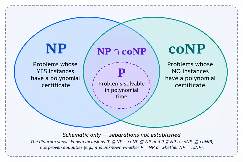
Equivalently, a problem belongs to NP if every YES instance has a certificate of polynomial length that can be verified in polynomial time.
For example, consider the integer factorization problem: given an integer N, can we find a non-trivial divisor of N?
Finding a divisor may be computationally expensive, but given a candidate divisor d, checking whether d divides N is straightforward and takes polynomial time.
Using our ideal-parallelism analogy, a nondeterministic machine can explore all candidate certificates simultaneously and accept if at least one is valid.
Every problem in P also belongs to NP (at worst the P problem itself is the desired polynomial certificate):
P ⊆ NP
Whether this inclusion is strict is one of the most important open questions in computer science.
coP and coNP
The complement of a decision problem is obtained by exchanging its YES and NO answers.
- coP: The class of complements of problems in P. Since a deterministic polynomial-time algorithm can simply reverse its answer, coP = P.
- coNP: The class of complements of problems in NP. Equivalently, a problem belongs to coNP if every NO instance has a polynomial-size certificate that can be verified in polynomial time.
A problem belongs to NP ∩ coNP if both YES and NO instances have polynomially verifiable certificates.
We know that P ⊆ NP ∩ coNP, but whether NP=coNP remains unknown.
PRIME, COMPOSITE, FACTOR and FACTORING
Integer factorization provides an interesting example of the difference between decision and search problems:
- PRIME: Given an integer N, is it prime? This problem belongs to P, thanks to the deterministic polynomial-time AKS algorithm (2002).
- COMPOSITE: Given an integer N>1, does it have a non-trivial divisor? This is simply the complement of PRIME, so it also belongs to P. We can determine whether a number is composite without knowing any of its factors.
- FACTOR: Given integers N and k, does N have a divisor d such that 1<d≤k? This decision problem belongs to NP ∩ coNP, but is not known to belong to P (NP requires just d, coNP requires the whole factorization of N and primality test of each factor).
- FACTORING: Given an integer N, find its prime factorization. This is a search problem, not a decision problem. No general classical polynomial-time algorithm is known, although subexponential algorithms exist.
Interestingly, FACTOR and FACTORING are polynomial-time equivalent in the sense that an efficient algorithm for either one would yield an efficient algorithm for the other. Given a polynomial-time algorithm for FACTOR, we could find divisors by binary search on k, then recursively factor the resulting integers.
This example illustrates an important distinction: a problem may have efficiently verifiable certificates for both YES and NO answers without having a known polynomial-time algorithm to solve it.
In other words, belonging to NP ∩ coNP does not imply that a problem belongs to P (at least, no such implication has been proved). This leads naturally to the broader question of whether efficient verification always implies efficient computation.
P vs NP
The P vs NP problem asks whether every decision problem whose YES solutions can be efficiently verified can also be efficiently solved.
We know that:
P ⊆ NP
But whether this inclusion is strict remains unknown:
P = NP?
If P = NP, polynomial-time verification would imply polynomial-time solution. Moreover, for standard NP problems, we could also construct a valid certificate in polynomial time rather than merely deciding whether one exists.
This does not mean that such algorithms would necessarily be simple to discover or practical to execute: polynomial-time algorithms can still have enormous exponents or constants.
Polynomial-Time Reductions
A polynomial-time reduction transforms an instance of problem A into an instance of problem B in polynomial time, preserving its YES/NO answer.
We write:
A ≤ₚ B
This means that a polynomial-time algorithm for B would also give us a polynomial-time algorithm for A.
Reductions allow us to compare the computational difficulty of different problems. However, polynomial-time reductions are not always appropriate: when studying finer complexity classes, we may need more restrictive reductions, such as logarithmic-space reductions.
NP-hard and NP-complete
Polynomial-time reductions allow us to identify the hardest problems within a complexity class.
A problem is NP-hard if every problem in NP can be reduced to it in polynomial time. An NP-hard problem does not necessarily belong to NP: it may be a search problem, or even a decision problem outside NP.
A problem is NP-complete if it satisfies two conditions:
- It belongs to NP.
- It is NP-hard.
In other words, NP-complete problems are the hardest decision problems in NP, with respect to polynomial-time reductions.
An important consequence is that if any NP-complete problem can be solved in polynomial time, then P = NP.
Conversely, if P ≠ NP, no NP-complete problem belongs to P.
Once we know that a problem A is NP-complete, we can prove another problem B is NP-hard by constructing a polynomial-time reduction A ≤ₚ B. If B also belongs to NP, then B is NP-complete.
The most famous example is SAT, the Boolean satisfiability problem, whose NP-completeness was established by the Cook–Levin theorem. We will examine SAT and the idea behind this proof in a separate article.
An example of an NP-hard problem that does not belong to NP is Generalized Chess: given a position on an arbitrarily large chessboard, determine whether the player to move has a forced win.
This problem is EXPTIME-complete, meaning that it is at least as hard as every problem solvable in exponential time. Since NP ⊆ PSPACE ⊊ EXPTIME, we know that Generalized Chess is outside NP.
Unlike ordinary NP problems, finding a winning strategy may require considering every possible response from the opponent.
Parallel Computation and NC — Nick’s Class
Before concluding, I would like to briefly introduce another interesting complexity class, NC, which concerns problems that can be efficiently parallelized. We will explore parallel computation in more detail later, but it seems worth mentioning here.
As discussed in the article on computational models, an ideal PRAM with exponentially many processors could explore all possible certificates of an NP problem simultaneously. However, this would require exponentially many computational resources.
NC (Nick’s Class) contains decision problems solvable in polylogarithmic parallel time, O(logᵏ n) for some constant k, using a polynomial number of processors.
For example, the sum of n integers can be computed using a tree of parallel additions, reducing the number of addition steps from O(n) sequentially to O(log n) in parallel.
Equivalently, NC can be characterized using uniform Boolean circuits of polynomial size and polylogarithmic depth.
Since a polynomial number of processors can be simulated sequentially with polynomial overhead, we know that:
NC ⊆ P
However, whether NC = P remains unknown.
This raises an interesting question: are there problems that can be solved efficiently by a sequential algorithm, but cannot be efficiently parallelized?
P-complete Problems
A problem is P-complete if it belongs to P and every problem in P can be reduced to it using suitably restricted reductions, typically logarithmic-space reductions.
Why not use ordinary polynomial-time reductions? Because every problem in P can be reduced to any non-trivial problem in P using a polynomial-time algorithm: we could simply solve the original problem during the reduction. Such reductions would therefore tell us nothing useful about parallel complexity.
Logarithmic-space reductions are more restrictive and can themselves be computed efficiently in parallel.
A standard example of a P-complete problem is the Circuit Value Problem (CVP): given a boolean circuit and the values of its inputs, determine whether its output is TRUE.
The circuit can be evaluated sequentially in polynomial time, but no general algorithm is known that evaluates arbitrary circuits in polylogarithmic parallel time using only polynomially many processors.
If any P-complete problem belongs to NC, then:
NC = P
Thus, P-complete problems are considered candidates for problems that are efficiently solvable sequentially but inherently difficult to parallelize.
This gives us an interesting analogy:
- NP-complete problems help us investigate whether P = NP.
- P-complete problems help us investigate whether NC = P.
In both cases, proving that a single complete problem belongs to the smaller class would establish equality between the two classes.
About Space Complexity
So far, we have classified computational problems mainly by the time required to solve them. However, we can ask a similar question about space complexity: how much memory does an algorithm need?
Just as with time complexity, we can define complexity classes based on the amount of memory available to deterministic or nondeterministic machines.
Some important examples are:
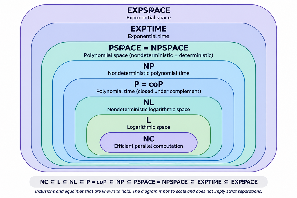
- L (Logarithmic Space): Problems solvable by a deterministic machine using O(log n) working memory.
- NL (Nondeterministic Logarithmic Space): The nondeterministic counterpart of L.
- PSPACE (Polynomial Space): Problems solvable by a deterministic machine using polynomial working memory.
- NPSPACE (Nondeterministic Polynomial Space): The nondeterministic counterpart of PSPACE. Interestingly, NPSPACE = PSPACE, as established by Savitch’s theorem.
- EXPSPACE (Exponential Space): Problems solvable using exponential working memory.
An interesting difference from time complexity is that polynomial space can be much more powerful than polynomial time: an algorithm may use only a polynomial amount of memory while taking exponentially many steps.
We know that:
L ⊆ NL ⊆ P ⊆ NP ⊆ PSPACE ⊆ EXPTIME ⊆ EXPSPACE
Several of these inclusions are not known to be strict.
Space complexity deserves its own discussion, so we will leave these classes aside for now. They are just as interesting as time complexity, and they reveal another important dimension of computational difficulty.
Conclusions
We have introduced some of the main computational complexity classes and the relationships between them:
- P: Decision problems solvable in polynomial time by a deterministic machine.
- NP: Decision problems whose YES answers can be verified in polynomial time, or equivalently, solved in polynomial time by a nondeterministic machine.
- coNP: Decision problems whose NO answers can be verified in polynomial time.
- NC: Problems that can be efficiently parallelized, using a polynomial number of processors and polylogarithmic time.
- NP-complete: The hardest problems in NP, with respect to polynomial-time reductions. They are candidates for problems that cannot be solved in polynomial time: if even one belongs to P, then P = NP.
- P-complete: The hardest problems in P, with respect to logarithmic-space reductions. They are candidates for problems that cannot be efficiently parallelized: if even one belongs to NC, then NC = P.
Two fundamental questions remain open:
P = NP?
NC = P?
The first asks whether every efficiently verifiable problem can also be efficiently solved. The second asks whether every efficiently solvable problem can also be efficiently parallelized.
In future I would like to describe SAT, one of the most important NP-complete problems, and understand why it is NP-complete through the ideas behind the Cook–Levin theorem. From there, we could move on to 3-SAT, or maybe on the Exponential Time Hypothesis, or on relation between classes.
In reality I would like to study FACTOR or interesting lower bounds for NP-complete problems, but so far I obtained my target that was simply reload again on my mind the previous definitions.